Lab 6 - Orientation Control

1. Prelab

To set up a robust system for debugging the PID controller, I plan to send gains for my PID controller each time I run a closed-loop command. For this lab, I plan to send information for Kp, Ki, Kd, and the amount of time the robot is commanded before the robot “times out” and stops. This allows the robot to stop after a specified period of time whether or not the robot has Bluetooth connection.

This can be done by using the ble.send_command function in Python, which allows new gains to be updated each time without needing to upload new code. The following Arduino code shows the framework of the command for this lab:

Whenever a closed-loop command is requested, debugging data is stored in arrays and is then sent to a notification handler. The time-stamped debugging data that I chose to collect are sensor data from the IMU and the outputs of each branch from the PID controller.

2. Lab Tasks

PID Input Signal

To get an estimate of the orientation of the robot, the gyroscope data myICM.gyrZ() will be integrated over time.

While integrating gyroscope data has low noise, the problem that arises is that the readings will drift over time. To minimize this error, the onboard digital motion processor built into the IMU can be used to minimize yaw drift. However, after conducting multiple tests of periods of 10 seconds, there was minimal drift observed, so I did not make implement any solutions to minimize yaw drift.

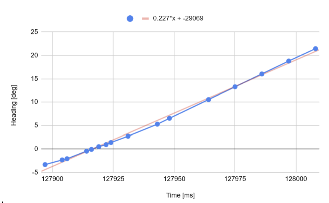
IMU data is sampled at a very quick rate compared to the ToF sensors. In a 10 second period, 1329 samples were taken, which is an average of 7.5 ms per heading update and equal to 133 Hz. From the below test, the fastest angular velocity occurred between the timestamps of 127897 ms and 128008 ms. During this period of time, the maximum angular velocity was measured to be 227 degrees/sec.

The IMU can be programmed to measure up to +/- 2000 deg/sec, which is sufficient for our applications. This parameter can be configured to decrease the maximum angular velocity to +/- 250 deg/sec, +/- 500 deg/sec, or +/- 1000 deg/sec by editing the GYRO_FS_SEL parameter.

Derivative Term

Taking the derivative of a signal that is the integral of a another signal can create induced errors. Differentiation amplifies high-frequency noise, so if the integrated signal has a small amount of noise, the derivative controller can become very noisy. In addition, because integrators can introduce drift over time, a derivative controller will create inputs based on the skewed data. Therefore, implementing a derivative controller based on an integrated signal will be difficult. Instead of using error, the derivative term can be calculated by using the raw measurements from the IMU and multiply the readings by Kd.

If error was used for the derivative term, a quick change in the error can cause a derivative kick. By using raw measurements instead, kick can be eliminated. Similar to lab 5, a LPF can be implemented to smooth the data to make the derivative controller more stable.

Programming Implementation

In the prelab section, I can send new gains and inputs to the Artemis over Bluetooth without needing to upload new code to the Artemis. This will allow any setpoints that need to be sent to the Artemis to be changed in real time allowing the robot to change headings or stop from objects at different distances.

The orientation of the robot can be controlled while the robot is driving forward or backward. This can be done by calculating a differential PWM value needed to rotate the robot and adding that input to the translational output of each motor. Two different PID loops will need to be implemented in which each controller will calculate PWM values and then summed together to create an output.

PI Controller

For this lab, I decided to use a PI controller as it was easier and quicker to tune than a PID controller. Because the robot returns back to its initial heading quickly without significant overshoot after tuning Kp and Ki, I decided that Kd was not needed in this case.

The strategy that I used to tune the controller was to first set Kp to an aggressive gain of 10 in which the robot oscillates around the initial heading of 0 degrees after receiving a large disturbance. Kp was brought down until the robot does not oscillate anymore after receiving a disturbance. After Kp is set, Ki was slowly increased until there was almost no steady state-error after the robot is disturbed. The values of the PI controller are Kp = 2.4, Ki = 6.85.

The following code shows the implemented PI controller:

The following video demonstrates the implementation of the PI controller:

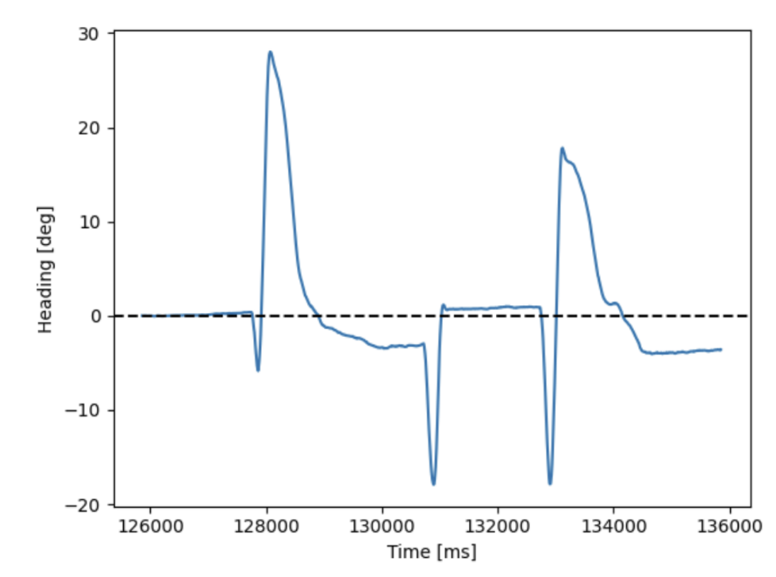
The largest steady-state error measured is ~3.5 degrees.

Tasks for 5000-level students

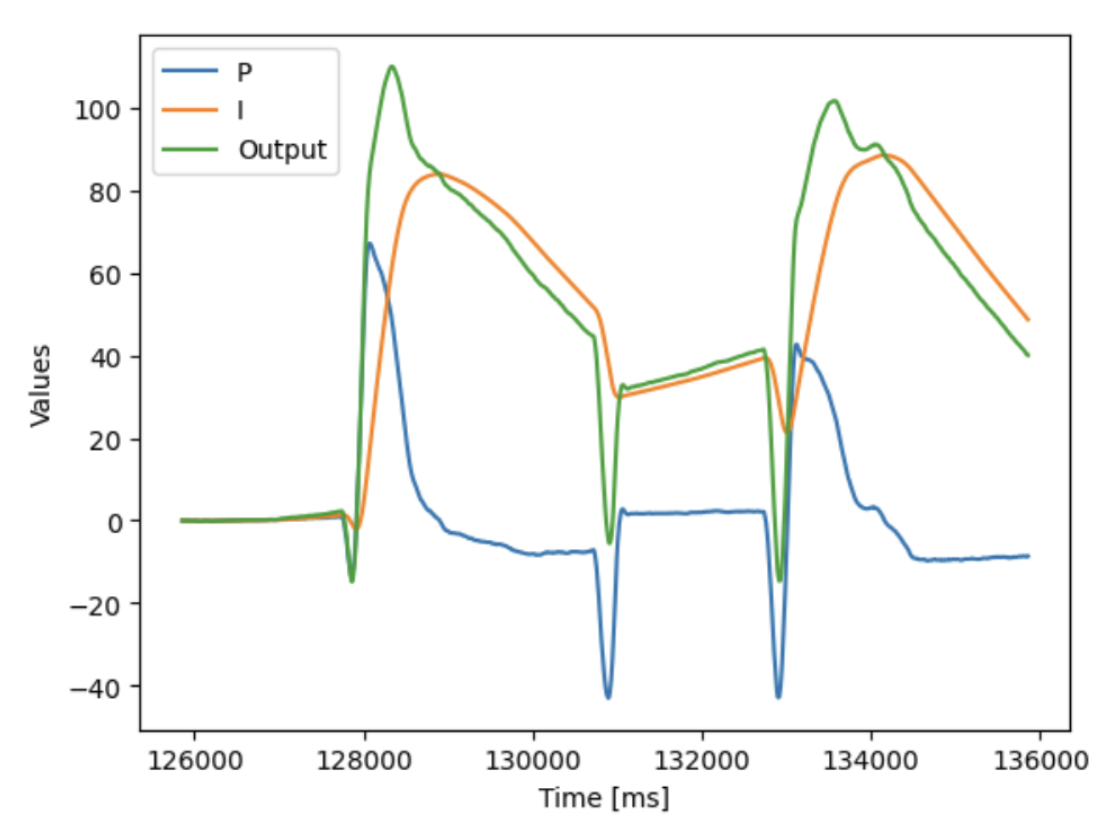
Integrator windup protection is required to prevent PI/PID controllers from accumulating massive, excessive error signals when actuators saturate. This was implemented in my controller by creating a limit on how much the integrator controller can contribute to the overall output of the PI/PID controller.

A clamp value of 100 was chosen, which helped limit the strength of the integrator controller. Without windup protection, the integrator controller dominates the PI loop and causes the vehicle to overshoot the setpoint. While the above video and figure does not show the integral controller saturating, the clamp value of 100 was determined experimentally with large disturbances to prevent wheel slip which allows the robot return to its initial heading quicker.

Collaborators

For Lab 5, I collaborated with Sean Zhen (sz378).