Lab 7 - Kalman Filter

1. Estimate drag and momentum

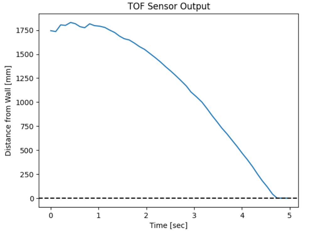
During this lab, the distance sensor will give incorrect distance data when placed too far from the wall, so the furthest the robot can be placed from a wall is ~1.75 meters.

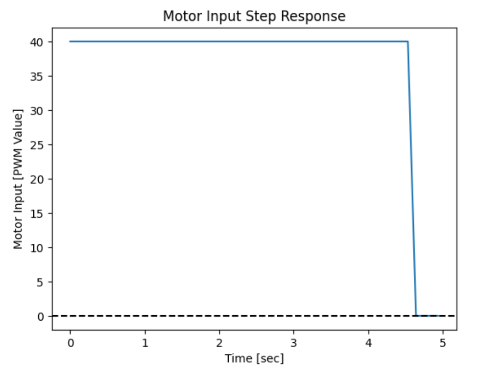
With this distance, for the robot to reach steady-state speed, I set the PWM value to 40, which is about 65% of the max PWM input obtained from lab 5.

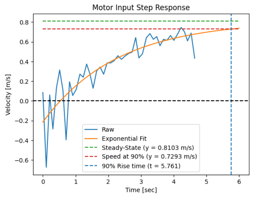
The steady-state speed is 0.8103 m/s, the 90% rise time is 5.761 seconds, and the speed at this rise time is 0.7293 m/s.

2. Initialize KF

From lecture, we know that the matrices A and B are defined as:

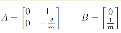
To find d, we can use the equation:

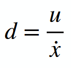
With u assumed to be 1 and steady-state velocity being 0.8103 m/s, d = 1 / 0.8103 = 1.234.

To find m, we can use the equation:

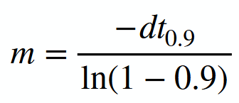
With the 90% rise time being 5.761 seconds, m = 3.0875

So, the A and B matrices are:

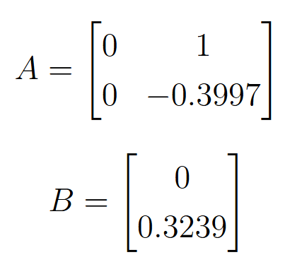
The sampling time in which a new distance measurement is obtained from the ToF sensor is 103 ms. The following code shows the discretized matrices along with matrix C and the state vector, x. Matrix C is [1,0] as the distance from the wall is positive.

For the Kalman Filter to work well, the process noise and sensor noise covariance matrices need to be specified. For process noise, with a sampling time of 103 ms, the standard deviation in position (sigma_1) is 31.16 mm, and the standard deviation in velocity (sigma_2) is 31.16 mm/s. For measurement noise, the ToF datasheet states that the short distance mode has an error of 20 mm, so sigma_3 is 20. The covariance matrices are implemented as shown:

3. Implement and test your Kalman Filter in Jupyter (Python)

Using the given Kalman filter example, the filter was implemented onto data from Lab 5:

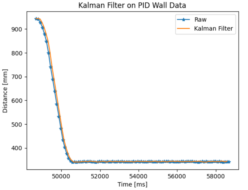
The Kalman filter seems to estimate the system state very well with a small lag. After increasing process noise to a standard deviation of 80 for sigma_1 and sigma_2, the filter trusts the measurements more than the model, and the time shift between the filter and raw measurements decrease.

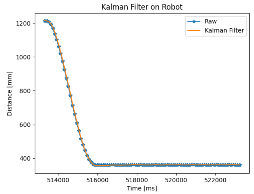
4. Implement the Kalman Filter on the Robot

Using the same command from Lab 5 to have the robot stop at the wall, the following code snippets were added into the command to implement the Kalman filter.

Tha Kalman filter was able to estimate the state of the robot very accurately. With the Kalman filter in place, I was also able to run a more aggressive PID controller than lab 5.

Collaborators

For Lab 7, I referenced Aidan Derocher’s work.