Lab 9 - Mapping

1. Control

For this lab, I will implement method 3 by creating a PID controller controlling the angular speed of the robot based on raw gyroscope values.

The goal of this lab is to obtain at least 14 readings per location. Due to the relatively fast frequency that the ToF sensor updates, I was able to obtain ~50 readings within 5 seconds of rotating, which is about 72 degrees per second. Because gyroscope values are very sensitive to the smallest changes in orientation, a low pass filter. An alpha value of 0.1 was used, which smoothed the gyroscope data and thus caused the PID controller to be smoother. Any lower values of alpha will cause the PID controller to fall behind and not respond fast enough.

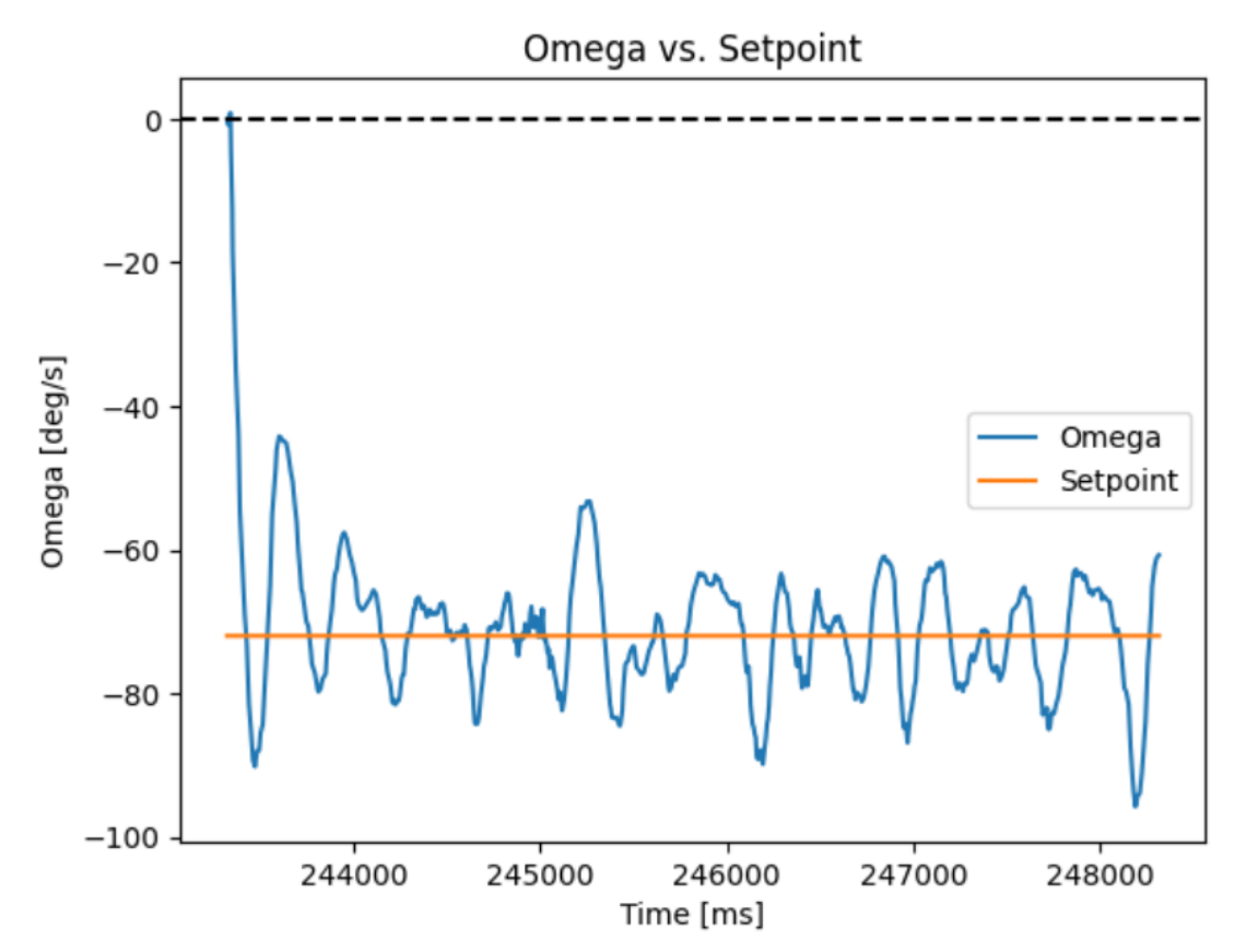
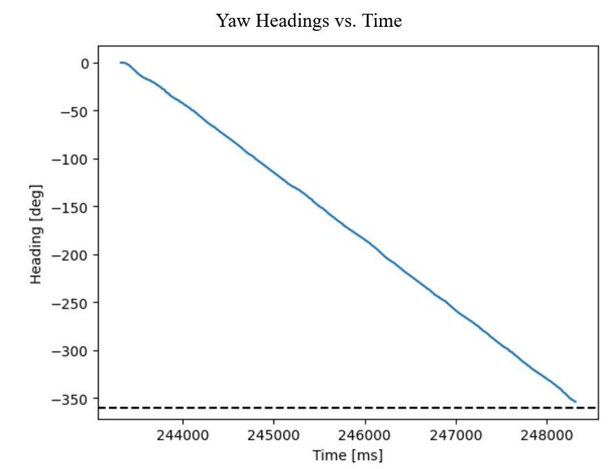
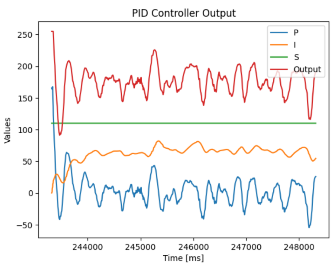
The above figures shows that the robot is able to make the full 360-degree turn in a five-second period. A PI controller with a static gain (Ks) was used to maintain an angular velocity of 72 degrees/sec. Ks was chosen to be 110, which is the minimum PWM value that causes the robot to start rotating. A static gain was included to reduce the overshoot from the proportional controller and quickly get the robot rotating.

The above figures also shows the output of the PI controller oscillating about the setpoint. This was due to the rough and wavy texture of the wood laminate flooring the robot was rotating on, which causes the proportional controller to increase significantly when it is caught on a crease of the flooring. The following video shows the robot completing the 360-degree turn on the laminate flooring.

The slowest speed that I was able to achieve was 72 degrees/second. Any angular velocity that is lower would cause the PID controller to oscillate violently despite having low Kp values. More details are included in the discussion section of this write-up. Because ToF measurements are collected at ~10 Hz, the robot rotates ~7.2 degrees between each measurement. If the robot was spinning in a middle of a 4x4 meter square room, the accuracy is +/- 3.6° (0.0628 rad). With the furthest distance being 2.83 meters (corner of the room), the error can be +/- 17.78 cm.

2. Read out Distances

Using the marked locations in the lab space, I placed my robot and collected distance sensor readings at (-3,-2), (0,0), (0,3), (5,3), and (5,-3). At each location, the robot faced in the -y direction (south) at the start with this direction marked as 0°.

The gyroscope has a sensitivity tolerance of +/- 1.5%, so with a rotation rate of 72 degrees/sec, the gyroscope can have an error of +/- 1.08 degrees/sec. Because the robot is rotating for five seconds to make a full 360 degrees, accumulated errors can be up to 5.4 degrees. This is only the calculated error based on gain error, so there are different errors, such as zero-rate output bias that can add up to +/- 5 degrees/sec. Because of this, the robot behavior is not reliable enough to assume that the readings are spaced equally in angular space, so gyroscope values will be used to create maps at each location.

Assuming that the robot is rotating on-axis, polar plots are created at each location:

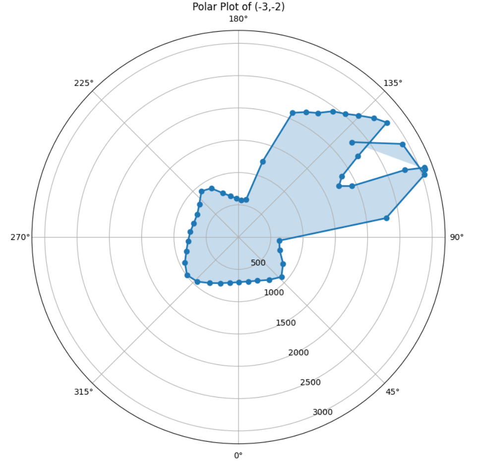
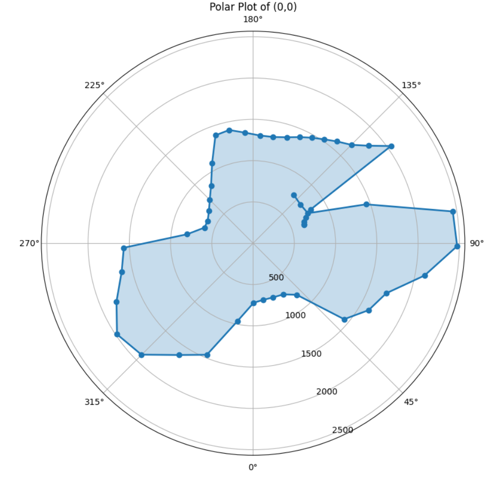
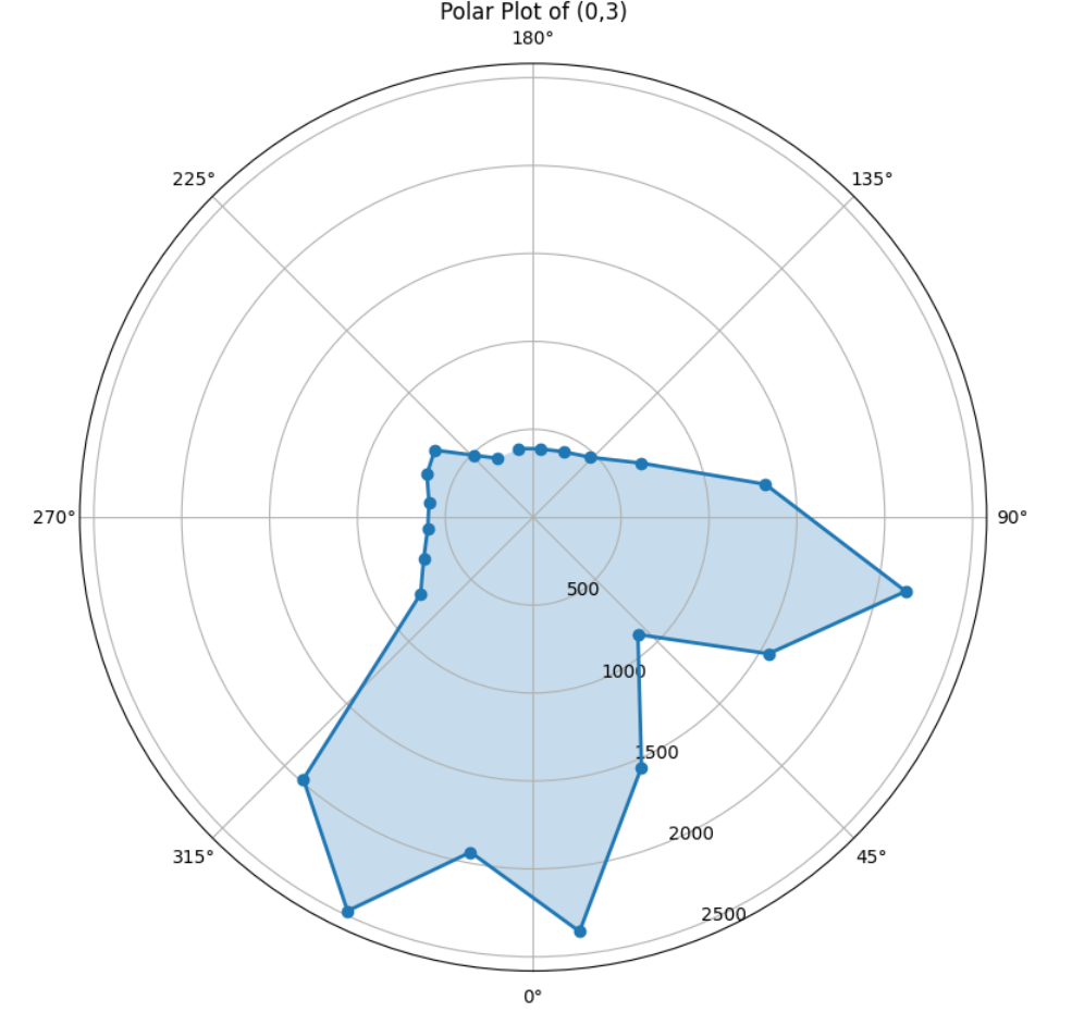
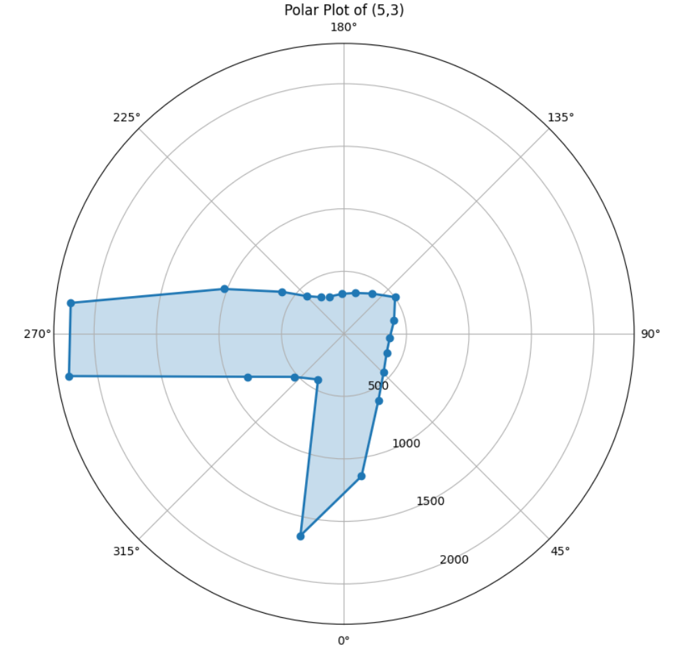
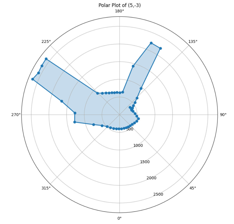
Due to some erroneous measurements, some data points were removed from locations (5,3) and (0, 3). Despite removing these points, the right-angle corners are clearly visible in each polar plot, so these measurements were not retaken (due to time constraints). The measurements in each polar plot match to what I expect.

To show the precision of the scans, I measured twice on the location (0,0):

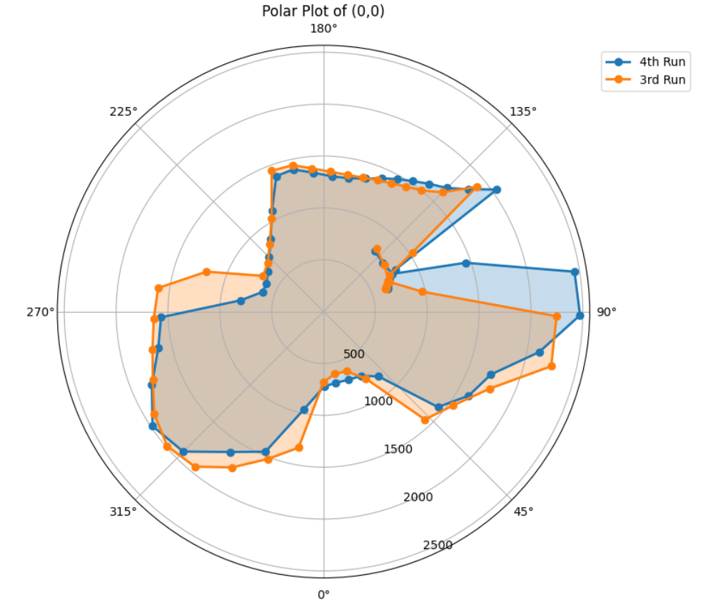
Between the two scans, the distance sensor readings match very closely throughout the entire 360° range. The largest variations are seen between the headings of 90° and 135° in which these measurements correspond to farther distance readings. Measurement readings that are closer range have little variation between the two scans.

3. Merge and Plot your Readings

There are three relevant coordinate frames:

1. Inertial frame (the world/room) that is centered at (0,0) and fixed to the room
2. Robot frame that is centered at the robot’s sensor, with +X corresponding to the robot’s right, and +Y corresponding to the robot’s front.
3. Sensor frame that indicates the position of the sensor. The sensor is placed at thr front-center of the robot and faces in the robot’s +Y direction with no rotation relative to the robot frame. The sensor is placed 82.5 mm from the center of the robot.

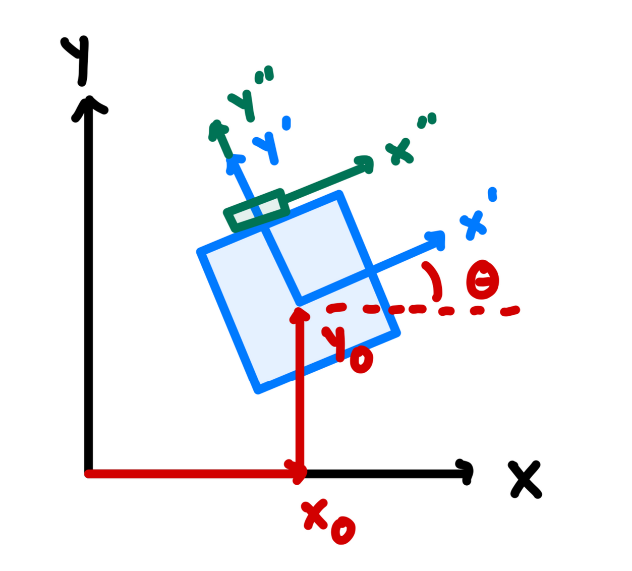
x_0 and y_0 represents the robot’s position relative to the inertial frame, with θ corresponding to the robot’s rotation. d_m represents the distance measurement from the ToF sensor.

To transform ToF measurements and heading orientation values into coordinates of the walls in the inertial frame (P^I), the following transformation needs to be done. T_R^I represents the transformation matrix from the robot frame to the inertial frame, T_S^R represents the matrix from the sensor frame to the robot frame, and P^S represents the distance sensor readings.

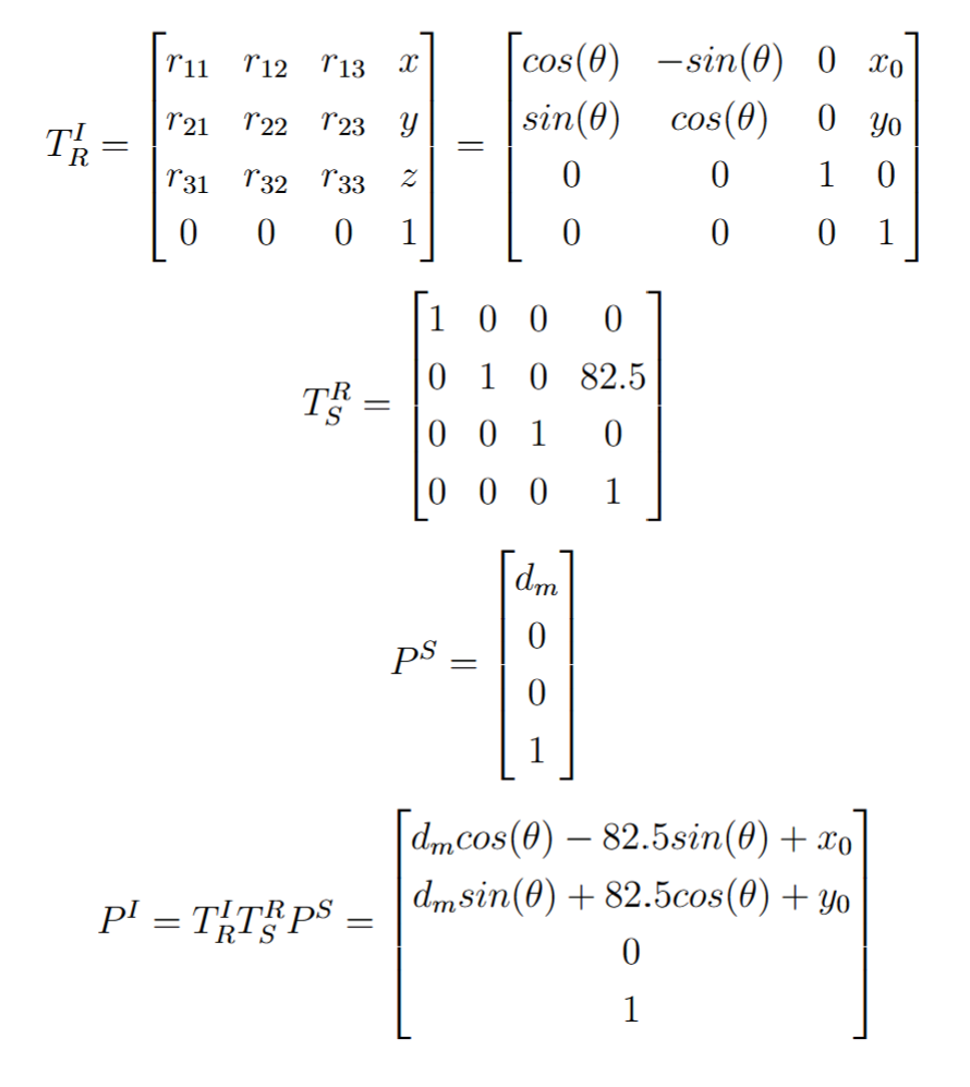
To make this transformation in Python, I used Sean Zhen’s function with the relevant variables:

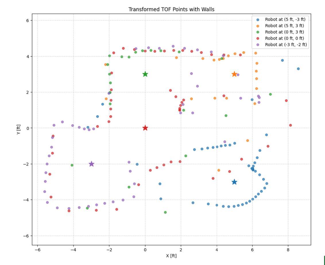
4. Convert to Line-Based Map

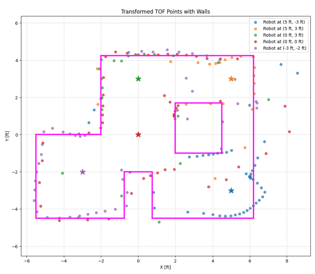
The transformed ToF coordinates give a very well-defined map for most regions. For ToF measurements when the robot is at (5,-3), there seems to not be a well-defined right-angle corner at the southeast corner, which can be caused by accumulated gyro errors. To fix this, ToF coordinates from other locations were used to estimate the positions of the right-most and south-most walls of the “world.” There are also some points that exceed the world boundaries but are associated with far distance readings that can be inaccurate, so those points are ignored and not used to draw the walls.

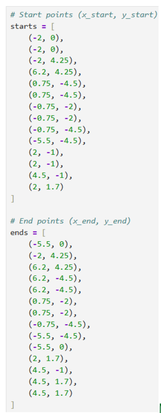
The two lists containing (x_start, y_start) and (x_end, y_end) are:

Discussion

I initially started with method 2, however, the PID loop was difficult to tune as it was sensitive to battery voltage and the friction of the floor. The PID controller was tuned on an Upson Hall floor but produced unsteady results within the Tang Hall lab. While method 2 would be more reliable as points are taken with the robot stationary, method 3 was ultimately used. This is why I had to submit this lab one day late. Method 3 had some errors with some erroneous measurements that had to be post-processed and removed. This is most likely due to the robot rotating at relatively high speed of 72 degrees/second. If the targeted angular velocity was lower, such as 20 degrees/second, the smallest PWM input (with a very low Kp value < 0.01) created an overestimated angular velocity and causes the controller to jitter the robot, which created inconsistent results. Thus, I made the robot rotate at 72 degrees/second as more than 14 readings was easily obtained at each location.

Collaborators

For Lab 9, I worked with Sean Zhen.