Lab 11 - Localization on the Real Robot

Setting up the Observation Loop

In this lab, the robot will be placed on four different locations in the map and will need to collect ToF sensor readings that are 20 degrees apart. This is similar to Method 2 from Lab 9.

To aid in the completion of this lab, I used Sean Zhen’s implementation of Method 2 from Lab 9 to have the robot make 20-degree turns and take a ToF measurement at the end of each turn. The PID loop is specifically tuned for my robot in which the values of Kp = 1.5, Ki = 45, Kd = 1, and a static gain of Ks = 100 were used to complete the 18 measurements. The following figures shows the precision of the PID loop completing each 20-degree turn.

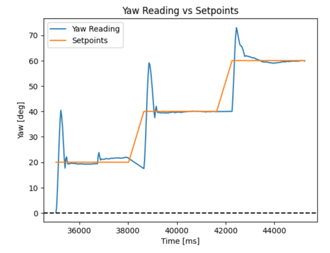
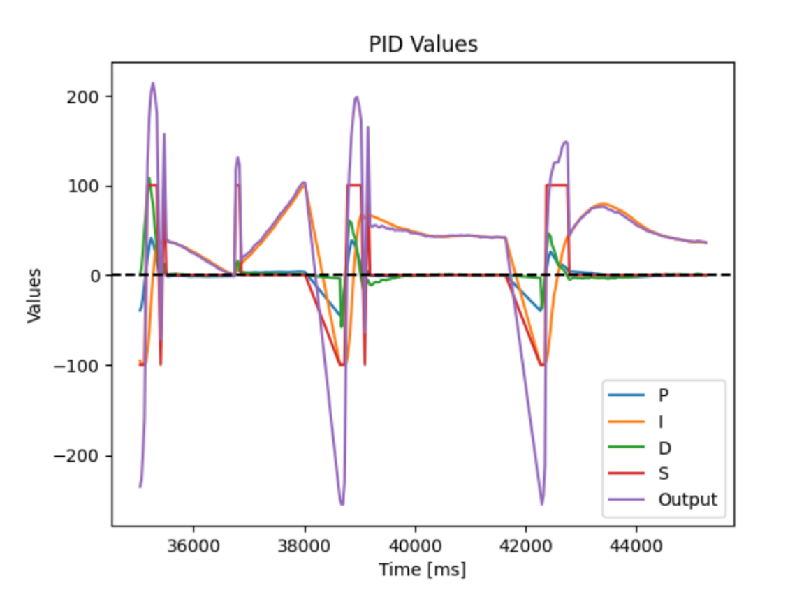
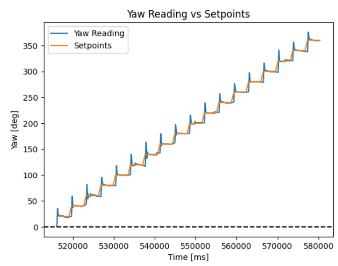
The implementation of the code is shown below:

The video below shows the robot conducting the 20-degree increment turns on the location (-3 ft, -2 ft, 0 deg).

1. Test Localization in Simulation

The notebook lab11_sim.ipynb was run, and the following figure is produced with the odometry, ground truth, and belief plotted on the map.

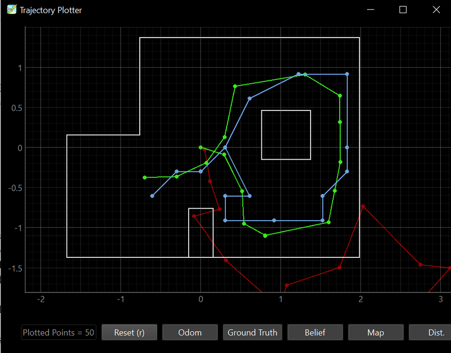
The belief follows closely to the ground truth, while the odometry drifts off the map.

2. Run the Update Step to Localize the Robot

2.1 Implement the function perform_observation_loop

For the function perform_observation_loop, an empty list for distance readings was first created in which a notification handler will receive the readings from the robot. asyncio.run(asyncio.sleep(3)) was used to ensure that the distance list becomes full before running loc.update_step() as the distance readings take time to populate through BLE. To make sure that the distance readings are in a format that can be used by the Bayes filter, the measurements need to be converted into meters and also as a type float.

2.2 & 2.3 Running the update step of the Bayes filter

At each location, the robot was placed facing in the +X direction. When collecting the 18 ToF measurements, I assumed that the robot is taking each measurement at equidistant headings. This makes the data collection for the Bayes filter simpler in which sensor_bearings can be set to as a numpy column array from 0 to 360 degree increments at 20 degree increments.

For each figure below, the ground truth and belief were plotted on the map at each location.

(-3 ft, -2 ft, 0 deg)

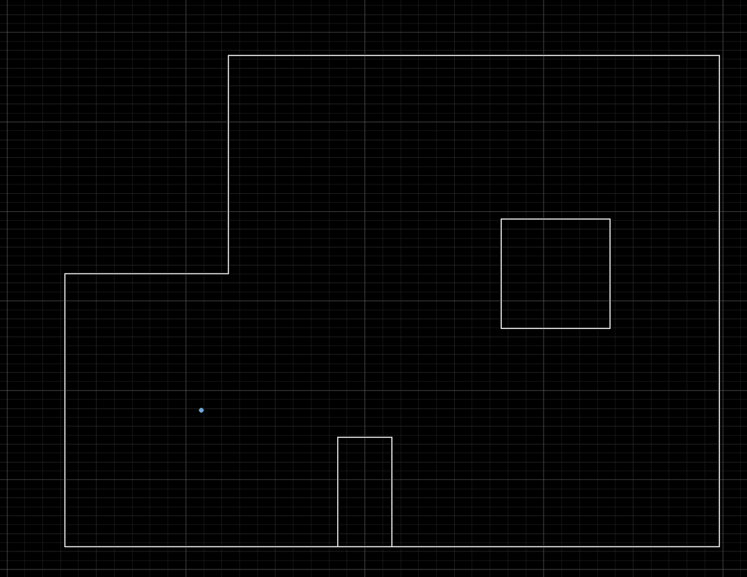
Sensor readings: [3040.0, 1792.0, 2847.0, 2096.0, 626.0, 691.0, 911.0, 897.0, 791.0, 783.0, 864.0, 1056.0, 837.0, 702.0, 692.0, 822.0, 880.0, 654.0]

Bel index: (np.int64(2), np.int64(2), np.int64(9)) with prob = 1.0

Bel_bar prob at index = 0.00051440329218107

Belief: (-0.914, -0.610, 10.000)

Ground Truth: (-0.9144, -0.6096, 0)

(0 ft, 3 ft, 0 deg)

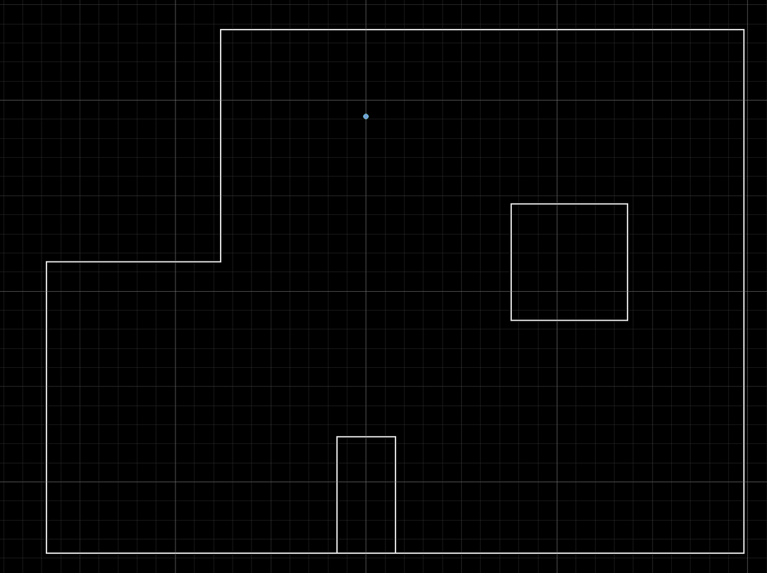
Sensor readings: [2202.0, 1053.0, 646.0, 446.0, 379.0, 405.0, 543.0, 738.0, 629.0, 646.0, 763.0, 2468.0, 2478.0, 2103.0, 2508.0, 982.0, 951.0, 2272.0]

Bel index: (np.int64(5), np.int64(7), np.int64(9)) with prob = 1.0

Bel_bar prob at index = 0.00051440329218107

Belief: (0.000, 0.914, 10.000)

Ground Truth: (0, 0.9144, 0)

(5 ft, -3 ft, 0 deg)

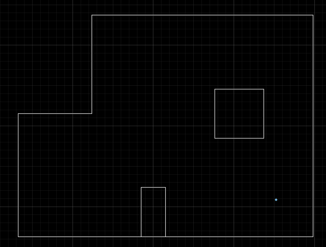
Sensor readings: [381.0, 415.0, 550.0, 906.0, 2349.0, 766.0, 846.0, 2781.0, 2925.0, 1287.0, 937.0, 499.0, 389.0, 338.0, 340.0, 381.0, 495.0, 420.0]

Bel index: (np.int64(10), np.int64(1), np.int64(9)) with prob = 0.9999999

Bel_bar prob at index = 0.00051440329218107

Belief: (1.524, -0.914, 10.000)

Ground Truth: (1.524, -0.9144, 0)

(5 ft, 3 ft, 0 deg)

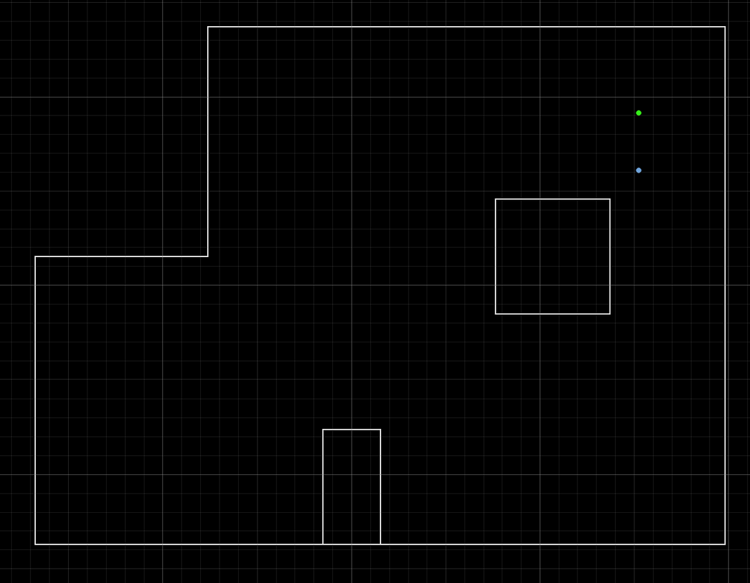
Sensor readings: [381.0, 427.0, 564.0, 453.0, 392.0, 427.0, 526.0, 860.0, 2117.0, 2248.0, 611.0, 431.0, 434.0, 2209.0, 1284.0, 590.0, 432.0, 370.0]

Bel index: (np.int64(10), np.int64(6), np.int64(9)) with prob = 0.9999999

Bel_bar prob at index = 0.00051440329218107

Belief: (1.524, 0.610, 10.000)

Ground Truth: (1.524, 0.9144, 0)

Discussion

At (-3 ft, -2 ft, 0 deg), (0 ft, 3 ft, 0 deg), and (5 ft, -3 ft, 0 deg), the X- and Y- coordinates of the belief was spot-on the ground truth with a +10 degree drift for heading.

At (5 ft, 3 ft, 0 deg), the belief was off by 1 cell in the y-direction with a difference of 0.3044 meters and a drift of +10 degrees.

To visualize the results, the sensor readings from each location is plotted on the map similar to Lab 9.

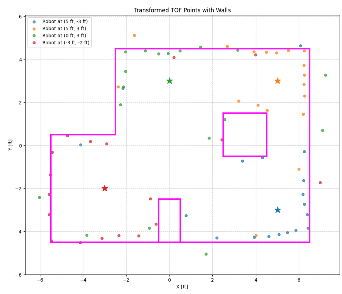
Out of the four marked poses, (5 ft, 3 ft, 0 deg) is the most ambiguous location on the map. This is because the robot is located near two long, orthogonal walls (north and east) that provide largely uniform distance measurements. Each other location has irregular geometry that crate distinct distance measurements. As a result, small changes in pose at (5 ft, 3 ft, 0 deg) can produce similar ToF readings, which will create localized poses that are more likely to be off from the ground truth.

Collaborators

For Lab 11, I worked with Sean Zhen, and I used his implementation of Method 2 from Lab 9 to complete this lab.